Losses and Metrics In Machine Learning

Reading Material¶

Note

We can prove mathematically that linear regression, logistics regression & all kinds of svms have a convex loss function hence only a single minima
All deep learning models with 2 or more layers can have a non Convex loss function hence more than one minima

Regression Losses¶

Loss Function	Use Case	Advantages	Disadvantages
Mean Absolute Error (MAE)	If your use case demands an error metric that treats all errors equally and returns a more interpretable value.	MAE is computationally cheap because of its simplicity and provides an even measure of how well the model performs.	MAE follows a linear scor- ing approach, which means that all errors are weighted equally when computing the mean. Because of the steepness of MAE, we may hop beyond the minima during backpropagation.
		MAE is less sensitive towards outliers	MAE is not differentiable at zero, therefore it can be challenging to compute gradients.
Mean Squared Error (MSE)	If the outliers represent significant anomalies, your use case demands an error metric where outliers should be detected.	MSE aids in the efficient convergence to minima for tiny mistakes as the gradient gradually decreases.	Squaring the values accelerates the rate of training, but a higher loss value may result in a substantial leap during back propagation, which is undesirable.
		MSE values are expressed in quadratic equations, aids to penalizing model in case of outliers.	MSE is especially sensitive to outliers, which means that significant outliers in data may influence our model performance.
Mean Bias Error (MBE)	The directionality of bias can be preserved with MBE. If you are simply concerned with a system’s net or cumulative behavior, MBE can help you assess how well biases balance out.	If you wish to identify and correct model bias, you should use MBE to determine the direction of the model (i.e., whether it is biased positively or negatively).	MBE tends to err in one direction continuously, while attempting to anticipate traffic patterns. Given that the errors tend to cancel each other out, it is not a suitable loss function for numbers ranging from (−∞, ∞)
Relative Absolute Error (RAE)	RAE is a method to measure the performance of a predictive model. If you are simply concerned and want a metric that indicates and compares how well a model works.	RAE can compare models where errors are measured in different units.	If the reference forecast is equal to the ground truth, RAE can become undefinable, which is one of its key drawbacks.
Relative Squared Error (RSE)	RSE is not scale dependent. If your use case demands similarity between models, it can be used to compare models where errors are measured in different units.	RSE is independent of scale. It can compare models when errors are measured in various units.	RSE is not affected by the predictions’ mean or size.
Mean Absolute Percentage Error (MAPE)	Since its error estimates are expressed in percentages. It is independent of the scale of the variables. MAPE can be used if your use case requires that all mistakes be normalized on a standard scale.	MAPE Loss is computed by standardizing all errors on a single scale of hundred.	As denominator of the MAPE equation is the predicted output, which can be zero leading to undefined value.
		As the error estimates are expressed in percentages, MAPE is independent of the scale of the variables. The issue of positive numbers canceling out negative ones is avoided since MAPE utilizes absolute percentage mistakes.	Positive errors are penalized less by MAPE than negative ones. Therefore, it is biased when we compare the precision of prediction algorithms since it defaults to selecting one whose results are too low.
Root Mean Squared Error (RMSE)	We can utilize RMSE if your use case necessitates a computationally straightforward and easily differentiable loss( as many optimization techniques do). Also, it does not penalize errors as severely as MSE does.	RMSE works as a training heuristic for models. Many optimization methods choose it because it is easily differ- entiable and computationally straightforward.	As RMSE is still a linear scoring function, the gradient is abrupt around minima.
		Even with larger values, there are fewer extreme losses, and the square root causes RMSE to penalize errors less than MSE.	The scale of data determines the RMSE, as the errors’ magnitude grows, so does sensitivity to outliers. In order to converge the model the sensitivity must be reduced, leading to extra overhead to use RMSE.
Mean Squared Logarithmic Error (MSLE)	MSLE reduce the punishing effect of significant differences in large predicted values. When the model predicts unscaled quantities directly, it may be more appropriate as a loss measure.	Treats small differences between small actual and predicted values the same as big differences between large actual and predicted values.	MSLE penalizes underestimates more than overestimates.
Root Mean Squared Logarithmic Error (RMSLE)	RMSLE has a significant penalty for underestimation than overestimation. If your use case requires situations where we are not bothered by overestimation, but underestima- tion is not acceptable, we can use RMSL	RMSLE is applicable at several scales and is not scaledependent. It is unaffected by significant outliers. Only the relative error between the actual value and the anticipated value is taken into account.	Due to RMSLE’s biased penalty, underestimating is penalized more severely than overestimation.
Normalized Root Mean Squared Error (NRMSE)	When comparing models with different dependent variables or when the dependent variables are changed, NRMSE is a valuable measure (log-transformed or standardized). It eliminates scale dependence and allows for easier comparison of models of different scales or even datasets	NRMSE overcomes the scale dependency and eases comparison between models of different scales or datasets.	NRMSE loses the units associated with the response variable.
Relative Root Mean Squared Error (RRMSE)	While the scale of the original measurements limits RMSE, RRMSE can be used if your use case necessitates comparing different measurement techniques. Also, RRMSE expresses the error relatively or in a percentage form.	RRMSE can be used to compare different measurement techniques.	RRMSE can hide inaccuracy in experiment results
Huber Loss	Huber Loss curves around the minima, which decreases the gradient and is more robust to outliers while optimally penalizing the incorrect values.	Linearity above the delta guarantees that outliers are given appropriate weightage (Not as extreme as in MSE). Addition of hyper parameter delta (δ) allows flexibility to adapt to any distribution	Huber loss is computationally expensive due to the additional conditionals and comparisons, especially if your dataset is huge.
		The curved form below the delta guarantees that the steps are the correct length during backpropagation.	To achieve the best outcomes must be optimized, which raises training requirements.
LogCosh Loss	Logcosh works similarly to mean squared error but is less affected by the occasional wildly incorrect prediction. It has all of the benefits of Huber loss; unlike Huber loss, It is twice differentiable everywhere.	As Log-cosh calculates the log of hyperbolic cosine of the error. Therefore, it has a considerable advantage over Huber loss for its’ property of continuity and differentiability.	It is less adaptable than Huber since it operates on a fixed scale (no δ).
		There are fewer computations required compared with Huber.	The derivation is more challenging than Huber loss and necessitates more research.
Quantile Loss	Use Quantile Loss when predicting an interval instead of point estimates. Quantile Loss can also be used to calculate prediction intervals in neural nets and tree based models, and It is robust to outliers.	It is robust to outliers.	Quantile loss is computationally intensive.
		It is beneficial for making in- terval predictions as opposed to point estimates. This func- tion can also be used in neural networks and tree based models to determine prediction intervals.	Quantile loss will be worse if we estimate the mean or use a squared loss to quantify efficiency

Issue with MAPE & Metrics which solve it

MAPE puts a heavier penalty on negative errors than on positive errors as stated in Accuracy measures: theoretical and practical concerns - REF As a consequence, when MAPE is used to compare the accuracy of prediction methods it is biased in that it will systematically select a method whose forecasts are too low. This issue can be overcome by using an accuracy measure based on the logarithm of the accuracy ratio (the ratio of the predicted to actual value). This leads to superior statistical properties and also leads to predictions which can be interpreted in terms of the geometric mean.

Mean Absolute Scaled Error (MASE) ,
Symmetric Mean Absolute Percentage Error (sMAPE)
Mean Directional Accuracy (MDA)
Mean Arctangent Absolute Percentage Error (MAAPE): MAAPE can be considered a slope as an angle, while MAPE is a slope as a ratio

Classification Losses¶

Multi Class Log-Loss or Categorical Cross Entropy

\[- \frac{1}{n}\sum_{i=1}^n \sum_{j=1}^C y_{ij}' log(p_{ij})\]

RecallCE Loss

\[RecallCE \ Loss = -\sum_{c=1}^C(1-R_{c,t})*log(p_{n,t}) \ = \ -\sum_{c=1}^C(1-\frac{TP_{c,t}}{FN_{c,t}+TP_{c,t}})*N_clog(p^{c,t}) \]

where $R_{c,t}$ is the recall for class c at optimization step t.

Classification Metrics¶

Accuracy, Precision, Recall, F1-score¶

Accuracy : What fraction of predictions were correct ?
Precision : What fraction of positive identifications were actually correct ?
Recall : What fraction of actual positives were identified correctly ?

Real Understanding

Precision and Recall are often in working against each other that is, improving precision typically reduces recall and vice versa. Try imagining a logistic regression model for a binary classification task and calculate Precision & Recall for different classification threshold. To understand this in more detail Schedule a Call

F1 score : The F1 score is the harmonic mean of the precision and recall.

Real Understanding

The highest possible value of an F-score is 1.0, indicating perfect precision and recall, and the lowest possible value is 0, if either precision or recall are zero. To understand this in more detail Schedule a Call

Fβ score : To consider recall β times as important as precision a modified
that uses a positive real factor β, where β is chosen such that recall is considered β times as important as precision, is:

ROC¶

AUC¶

Ranking Metrics¶

MRR¶

DCG¶

NDCG¶

Statistical Metrics¶

Correlation¶

Computer Vision Metrics¶

PSNR¶

SSIM¶

IoU¶

NLP Metrics¶

Perplexity¶

BLEU score¶

Inception score¶

Frechet Inception distance¶

Table of Confusion¶

Literally very confusing¶

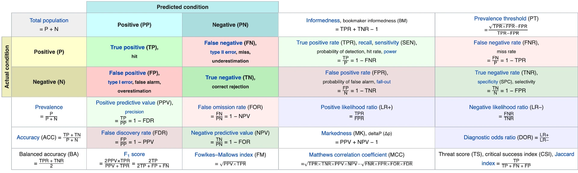
Condition positive (P) : the number of real positive cases in the data
Condition negative (N) : the number of real negative cases in the data
True Positive (TP) : A test result that correctly indicates the presence of a condition
True Negative (TN) : A test result that correctly indicates the absence of a condition
False Positive (FP) : A test result which wrongly indicates that a particular condition is present
False Negative (FN) : A test result which wrongly indicates that a particular condition is absent

Some basic formula¶


sensitivity, recall, hit rate, or true positive rate (TPR)	$\mathrm {TPR} ={\frac {\mathrm {TP} }{\mathrm {P} }}={\frac {\mathrm {TP} }{\mathrm {TP} +\mathrm {FN} }}=1-\mathrm {FNR}$
specificity, selectivity or true negative rate (TNR)	$\mathrm {TNR} ={\frac {\mathrm {TN} }{\mathrm {N} }}={\frac {\mathrm {TN} }{\mathrm {TN} +\mathrm {FP} }}=1-\mathrm {FPR}$
precision or positive predictive value (PPV)	$\mathrm {PPV} ={\frac {\mathrm {TP} }{\mathrm {TP} +\mathrm {FP} }}=1-\mathrm {FDR}$
negative predictive value (NPV)	$\mathrm {NPV} ={\frac {\mathrm {TN} }{\mathrm {TN} +\mathrm {FN} }}=1-\mathrm {FOR}$
miss rate or false negative rate (FNR)	$\mathrm {FNR} ={\frac {\mathrm {FN} }{\mathrm {P} }}={\frac {\mathrm {FN} }{\mathrm {FN} +\mathrm {TP} }}=1-\mathrm {TPR}$
fall-out or false positive rate (FPR)	$\mathrm {FPR} ={\frac {\mathrm {FP} }{\mathrm {N} }}={\frac {\mathrm {FP} }{\mathrm {FP} +\mathrm {TN} }}=1-\mathrm {TNR}$
false discovery rate (FDR)	$\mathrm {FDR} ={\frac {\mathrm {FP} }{\mathrm {FP} +\mathrm {TP} }}=1-\mathrm {PPV}$
false omission rate (FOR)	$\mathrm {FOR} ={\frac {\mathrm {FN} }{\mathrm {FN} +\mathrm {TN} }}=1-\mathrm {NPV}$
Positive likelihood ratio (LR+)	$\mathrm {LR+} ={\frac {\mathrm {TPR} }{\mathrm {FPR} }}$
Negative likelihood ratio (LR-)	$\mathrm {LR-} ={\frac {\mathrm {FNR} }{\mathrm {TNR} }}$
prevalence threshold (PT)	$\mathrm {PT} ={\frac {\sqrt {\mathrm {FPR} }}{{\sqrt {\mathrm {TPR} }}+{\sqrt {\mathrm {FPR} }}}}$
threat score (TS) or critical success index (CSI)	$\mathrm {TS} ={\frac {\mathrm {TP} }{\mathrm {TP} +\mathrm {FN} +\mathrm {FP} }}$
Prevalence	${\frac {\mathrm {P} }{\mathrm {P} +\mathrm {N} }}$
accuracy (ACC)	$\mathrm {ACC} ={\frac {\mathrm {TP} +\mathrm {TN} }{\mathrm {P} +\mathrm {N} }}={\frac {\mathrm {TP} +\mathrm {TN} }{\mathrm {TP} +\mathrm {TN} +\mathrm {FP} +\mathrm {FN} }}$
balanced accuracy (BA)	$\mathrm {BA} ={\frac {TPR+TNR}{2}}$
F1 score is the harmonic mean of precision and sensitivity	$\mathrm {F} _{1}=2\times {\frac {\mathrm {PPV} \times \mathrm {TPR} }{\mathrm {PPV} +\mathrm {TPR} }}={\frac {2\mathrm {TP} }{2\mathrm {TP} +\mathrm {FP} +\mathrm {FN} }}$
phi coefficient (φ or rφ) or Matthews correlation coefficient (MCC)	$\mathrm {MCC} ={\frac {\mathrm {TP} \times \mathrm {TN} -\mathrm {FP} \times \mathrm {FN} }{\sqrt {(\mathrm {TP} +\mathrm {FP} )(\mathrm {TP} +\mathrm {FN} )(\mathrm {TN} +\mathrm {FP} )(\mathrm {TN} +\mathrm {FN} )}}}$
Fowlkes–Mallows index (FM)	$\mathrm {FM} ={\sqrt {{\frac {TP}{TP+FP}}\times {\frac {TP}{TP+FN}}}}={\sqrt {PPV\times TPR}}$
informedness or bookmaker informedness (BM)	$\mathrm {BM} =\mathrm {TPR} +\mathrm {TNR} -1$
markedness (MK) or deltaP (Δp)	$\mathrm {MK} =\mathrm {PPV} +\mathrm {NPV} -1$
Diagnostic odds ratio (DOR)	$\mathrm {DOR} ={\frac {\mathrm {LR+} }{\mathrm {LR-} }}$
Confusion Matrix Reference

References¶

Focal Loss